Bayesian State Bar Passage

What are hierarchical models?

We start with a simple question: Which states have the lowest and highest bar passage rates? On the surface, this is simple arithmetic. Just divide the number of bar passers by the number of takers. And in a way, that’s all there is to it.

But in another context, it’s trickier. Let’s look at Alaska. In our data - spanning 2014 to 2017 - there are two takers and two passers; a bar passage rate of 100%. Do we assume their bar exam is fluff, and if I took it I would be sure to pass? If a thousand cold souls took it would they all pass?

Framing the issue so highlights what we really want to know. We want to know what I call the hypothetical pass rate with an infinite number of takers. Let’s call this the infinite takers pass rate. In other words, if a gazillion people took the Alaska bar, what percentage would pass? Surely it’s not 100%.

Alas, we can never know this number with certainty. Fortunately, only a small number of people are trying to become lawyers, so we will never know any state’s pass rate with a gazillion takers - its infinite takers pass rate. We can, however, estimate this rate - and a probability distribution of possible values for this rate - with a Bayesian hierarchical model.

Before looking at the hierarchical model, let’s look at two extreme ways to estimate a state’s infinite pass rate. First, we can simply say that the state’s estimated infinite pass rate is its real pass rate. We could also create confidence intervals for this rate by sampling from a binomial distribution that only contains the state’s takers and passers.

Let’s call this the no-pooling method, since we are not using any information outside the state to estimate the state rate. This makes sense on the surface, but the problem is that we are making an estimate based on a limited number of data points: limiting our data to the takers within a state. In a state like Alaska, with only two takers, this is a problem. Plus, with a pass rate of 100%, we are flipping a one sided coin that will always return heads.

At the other extreme, we might assume that the best guess for a state’s infinite takers pass rate is the United States pass rate. This gives us more data since we are using data outside the state to predict the state’s rate. With this approach, Alaska’s estimated pass rate is the US rate: 77%. This approach is called complete pooling because we are lumping all states together.

The benefit of this approach is that it gives us more data. Unfortunately, complete pooling arrives with its own squeaky wheel. States have different bar exams with different levels of difficulty. As a result, we can assume that states will have different infinite takers pass rates.

What if we can combine the best of both approaches? What if we primarily use the state’s own rate, but dip into the US rate to the degree that state data is lacking? This concept is called partial-pooling and it provides the backbone of hierarchical models.

To see how it works, let’s put on our jackets and go back to Alaska. With just two data points, we know almost nothing about it’s infinite takers pass rate. With this fog of almost-ignorance, our best guess might be the US rate.

But, let’s keep in mind we do have two Alaska test takers and they both passed. This is some, albeit slight, information. Given this, maybe we move our Alaska estimate a few percentage points higher than the US rate? This intuitive thought process encapsulates hierarchical methods.

Hierarchically modeling state bar passage rates

With this intuitive understanding of hierarchical models in mind, let’s start modeling.

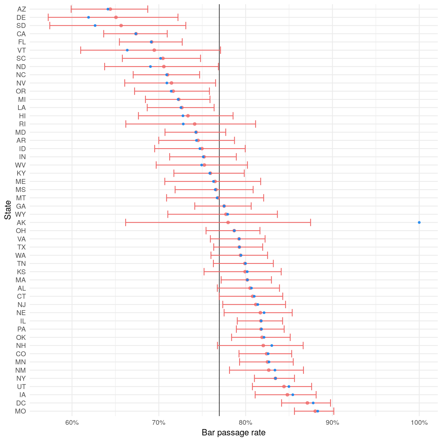
The plot below shows the results from a Bayesian hierarchical binomial model. The model is binomial because bar passage takes one of two values: pass or fail. The blue dots are the state’s actual pass rate, while red dots are the estimated pass rates. The red line represents the 90% highest posterior interval (HPI). The HPI is akin to the frequentist’s confidence interval. In fact, the HPI is what most people think a confidence interval means: there is a 90% chance that the true infinite takers pass rates falls within the 90% HPI.

The plot highlights a couple features of Bayesian hierarchical models. First, look again at Alaska. Confirming our intuition, the estimated infinite takers pass rate sits a few percentage points higher than the United States rate. Also, Alaska’s wide HPI indicates the lack of data points for the state.

Conversely, look at a state like California that has a lot of bar takers. Its estimated rate is almost identical to its actual rate. When a state has a lot of bar takers, there is less need to infer its estimated state rate from the United States rate. It can infer a pretty exact estimate from the state data alone.

Second, notice that states with actual pass rates higher than the United States average have estimated pass rates lower than their actual rates. And the opposite is true for states with actual pass rates lower than the United States average. This reveals how hierarchical models pull the estimated state rates towards the United States rate. More generically, hierarchical models pull the group estimates towards the global estimate.

Diving deeper: Estimating state passage rates based on LSAT scores and GPA

At this point, our temptation might be to look at the state with the lowest estimated bar passage rate and crown it as the state with the most difficult bar exam. But, this assumes that states have similar students taking their bar exams. For a host of reasons, this assumption might fail.

We can attempt to control for student quality by incorporating undergraduate GPA and LSAT scores into the model.

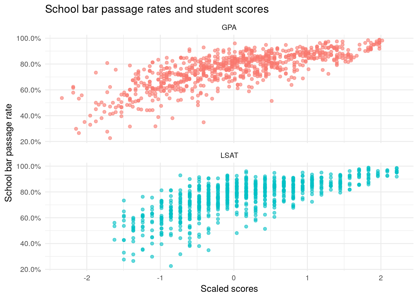
The plot below highlights the correlation between undergraduate GPA, LSAT, and bar passage. The values for GPA and LSAT are normalized to have a mean of zero and standard deviation of one, since this is what we will use for the model. The plot shows that a school’s average GPA and LSAT for its incoming students is positively related to bar passage, so each might be good candidate predictors for our bar passage model.

Now, let’s model this relationship. For reasons we won’t explore now, the best fitting model is one with LSAT and GPA, along with polynomial terms for LSAT and GPA.

The plot below shows each state’s predicted bar passage rate with average students. To get here, we first created a model of bar passage with state, LSAT, and GPA as predictors. Then, we created a test data set with 100 takers for each state, and each taker had an average LSAT and GPA. The average represented below is each state’s average pass rate from these 100 middle-of-the-road hypothetical takers.

The plot provides an estimate of what each state’s passage rate would have been if all takers in the state had an average LSAT and GPA. In this way, it attempts to make test-taker ability the same for every state. The blue dot is the average hypothetical pass rate, while the green dot is the actual pass rate. The blue line is the 90% HPI.

Theoretically, these rates should give us a better indicator of bar exam difficulty than the raw pass rate because they control for student ability.

There are always caveats with models

The last sentence notes that this is ‘theoretically’ a better indicator of bar exam difficulty. Let me fill in this theoretical gap. LSAT and GPA are provided as school averages in the data. But in the prediction model they are assumed to be individual scores. This can be problem if states have different LSAT and GPA distributions around the average.

Another issue is that the LSAT and GPA data is only broken down by school, not by state where students took the bar exam. For example, the University of Kentucky may have had students take the bar exam in three different states, but we do not have the average LSAT and GPA for each state’s takers from the University of Kentucky. We only have the overall school average for the University.

Therefore, another assumption is that LSAT and GPA scores within a school are evenly distributed between students who took the bar exam in different states from the school. Continuing with our example, we’re assuming that the LSAT and GPA distribution of students from the University of Kentucky who took the bar exam in Ohio is the same as student from the University who took the bar exam in Kentucky.

These two assumptions do not hold perfectly; and unfortunately, there is no way to test them. But, I’ll fall back on my favorite line in statistics, “All models are wrong, but some are useful.” Intuitively, I think the assumptions hold enough for the models to be useful.